Background Physics

Rocstar Multiphysics

In Rocstar there are two or more 3D physical domains abut at a common interface.

• The domains do not overlap
• The geometry of the interface is a 2D surface in space
• The domains may move/deform but they do not come apart

The two domains have differing physical character and interact at the interface.

• Mass, momentum, energy and charge are conserved in the interactions across the interface
• Some physical quantities of interest “jump” at the interface (e.g. density).

The interface may have physics of its own.

• The interface could be reactive with a combustion or other chemical process
• The interface could propagate or move due to some process
• Goal: Simulate two or more physical domains which interact across a moving, reacting interface
  

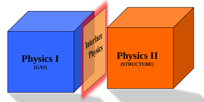
Each domain is simulated numerically by methods observing the respective physics.

• Rocstar implements a partitioned approach wherein each domain is simulated by a dedicated solver
• Rocstar solvers are independently developed and can stand alone as simulation applications in their own regard
• Rocstar uses staggered stepping (i.e. stepping is centrally synchronized)

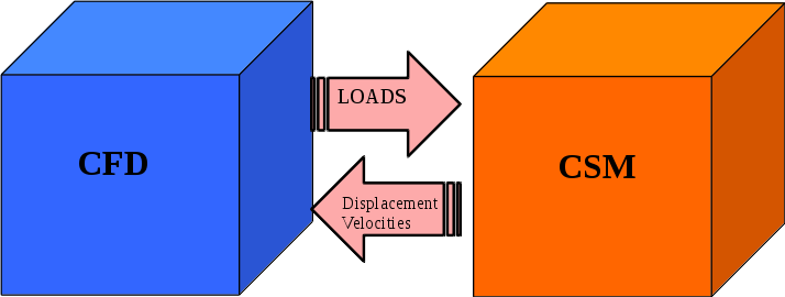
The next few images utilize a fluid structure interaction problem in order to adequately demonstration the physical capabilities of Rocstar.
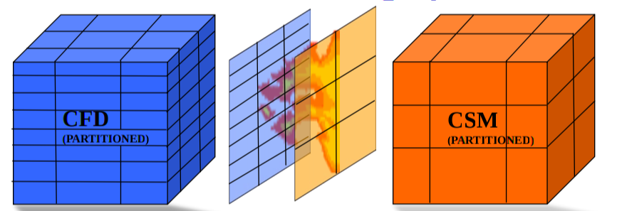
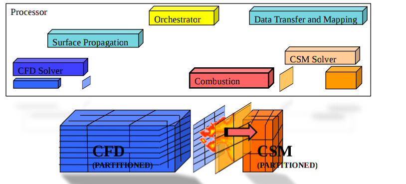
Partitioned and staggered: stepping and interactions are centrally synchronized

• Fluids domain steps and calculates pressure loads at the interface
• The loads are then passed to the structures domain
• The structures domain steps and calculates the deformation and interface velocities
• Interface motion sent to fluids domain
• The process is repeated to step the simulation through time
  

Each domain is decomposed into partitions to be distributed among processors.

• Rocstar’s solvers implement their own parallelism and partitioning
• In general, the partitioning is disparate across the domains
• In this example, 72 fluid partitions + 18 structures partitions implies 72 physical processors

The domains and shared interface are discretized by each solver application.

• Rocstar’s solvers each have their own mesh (i.e. non-conformal between interface discretizations).
• Each solver marches through time according to the domain-specific physics (i.e. time steps are disparate).
• Getting the interface data transfer right is essential for accuracy and stability of the simulation.
• The interface is reactive. It catches on fire, injects materials, and propagates (burns).
  • Combustion depends on solutions and geometry of other domains
  • Both geometries change drastically (propellant burns away completely!)
    

Each computer processor has one or more partitions of one or more solver’s domain.

• The geometry and data of each domain is spread out among all the processors in the simulation.
• Not all processors have a piece of all domains
• Not all processors have interface data
  

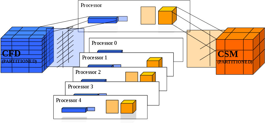
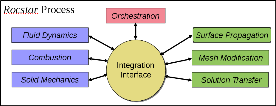
A simulation processor may have an instance of each solver, its domain, and interface. There must be a control flow manager for synchronous stepping, to handle some jump conditions, and unit conversions. To handle the burning, we need a combustion solver capable of operating on geometry and data from other solvers and their domains. We need sophisticated surface propagation capabilities to handle the interface motion due to burning. Mesh modification will be required for handling the extreme changes in geometry due to burning and deformations. Finally, all the pieces have to interact in an efficient manner, sharing data and methods, and working together to simulate the complete system.

The integration interface provides the mechanisms by which applications can publish and access methods and data. This is the “glue” of the Rocstar multiphysics simulation.

Physics Modules

Here is the Rocstar simulation suite architecture layout

Fluid Simulations

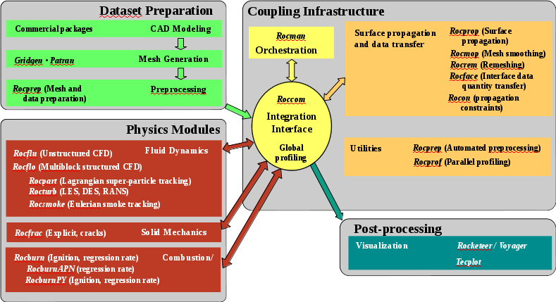
The governing Equations are based off of the unsteady, compressible, Navier-Stokes or Euler equations.

Fluid Dynamics: Rocflo	Unstructured mesh Fluids: Rocflu
1. Numerical Formulation	1. Mesh
a. Finite volume	a. Mixed tetrahedra, prisms, pyramids, hexahedra
b. Explicit Runge-Kutta
c. Arbitrary Lagrangian-Eulerian (ALE) method on moving meshes	2. Method:
d. 2nd order central scheme	a. Explicit, finite-volume, ALE
e. Roe upwind scheme	b. First or second order
	c. Higher order WENO scheme
2. Code Characteristics
a. Structured, multi-block mesh	3. Models
b. Plug-in modules for turbulence, particles, smoke, radiation	a. Lagrangian particles/super-particles
	b. Eulerian smoke
	c. Built-in propagation constraints
	d. Time-zooming

Fluid Simulations

Files Required

Both Rocflo and Rocflu require the same files, but have differences in format and naming

ASCII-format Gridgen mesh files produced:

	Rocflo	Rocflu
Mesh file	<casename>-PLOT3D.grd	<casename>-COBALT.inp
Boundary condition file	<casename>-PLOT3D.inp	<casename>-COBALT.bc

	Rocflo/Rocflu
Boundary Condition File	<casename>.bc
Input File	<casename>.inp

Gridgen to Rocstar boundary condition map file

Rocflo	Rocflu
<casename>-PLOT3D.bcmp	<casename>.cgi

Structural Dynamics

Structural Dynamics: Rocfrac
1. Large strains, rotations with Explicit/Implicit, ALE
2. Non-linear material models
a. Hyperelastic: Arruda-Boyce & Neo-Hookean
b. Non-linear constitutive laws: Viscoplastic & Porous viscoelastic
3. Mixed-enhanced elements
4. Transient thermal solver
5. Crack propagation
a. Cohesive elements allow failure
6. Stabilized and mixed displacement-pressure elements

Rocfrac Simulation

Files Required

Required Files	Filename
ASCII-format grid file produced by Patran	<casename>.out
ASCII-format input file	RocfracControl.txt

Rocburn

Combustion Module

RocburnAPN	RocburnPY
1. 1-D heat conduction into propellant	1. 1-D heat equation
2. Uses gas pressure power law	2. Dynamic heating
3. Provides regression rate for burning propellant	3. Geometrically dependent film coefficient
4. Burnout capabilities, no heating	4. Ignition modeling
	5. Burnout
	6. Provides aPn regression rate for burning elements
	7. Can use lookup tables

Required Files

Choose only one ASCII-format input file
RocburnAPNControl.txt
RocburnPYControl.txt

Please see the PhysicsModules powerpoint for the RocburnAPNControl.txt and RocburnPYControl.txt .

These sections are adapted from the Multiphysics and PhysicsModules powerpoints respectively.