 |
Rocstar
1.0
Rocstar multiphysics simulation application
|


|
|
Rocstar
1.0
Rocstar multiphysics simulation application
|
|
The Rocstar source code comes with a set of examples and test problems in the main source directory under Examples.
This section is adapted from the ACM Rocflu and ACM Rocflo presentation.
For information on setting up and running the Attitude Control Motor example problem please see the Rocstar Quickstart Guide. Running the problem as described in the Quickstart Guide can take a while to complete. To shorten the problem to run in a more timely fashion, make the following changes after following the directions in the Guide.
The goal of this example is to assemble and run a moving-boundary, fluid-combustion coupled problem using Rocflo and Rocflu. The problem consists of a small (2 inch) attitude control motor, which is represented using a block-structured hexahedral mesh. A key aspect of this simulation is the regressing buring surface.
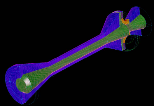
The motor is two inches long and it features fluid-combustion coupling. The fluid model has unstructured tetrahedral grid. The goal of this example is to assemble and run moving-boundary fluid-combustion coupled run with Rocflo.
First, using CAD software such as Pro/Engineer you export IGES format. Then you should be able to make simple geometries in Gridgen. Particularily for Rocflu, it is set unstructured mixed meshes. Meshes can be tets, hexes, prisms, and pyramids.
Now you need to set up NDA with grids and input files. Choose a "casename"; in this case it should be set ACM. Grid and boundary condition map files. Basic input, boundary conditions, controls files.
After all this gets done, we can preprocess and partition using Rocprep on NDA.
For Rocflu Boundary Conditions, following requirement should be met:
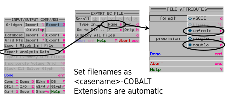
You can export COBALT mesh and BC files for Rocflu Grid. They folloing this format.
This example can be run in the same manner as the other examples discussed elsewhere. Follow the procedure from the Rocstar Quickstart Guide but using the following commands specific to this example. Rocprep is Rocstar's dataset preparation tool. It takes an initial dataset and pre-processes it accordingly for a given problem. Datasets that have not yet been preprocessed are referred to as Native Data Archives. Use the following command for rocprep:
All directories and paths mentioned below are within the data directory generated by running the rocprep command.
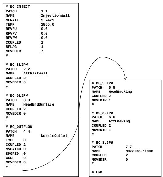
ACM.bc file resides at NDAs/Rocflu/Modin and "patch" defines Rocflu boundary condition. Patches correspond to Gridgen BC definitions on specific sections of the model. Following image is the example screen shot of ACM.bc file :
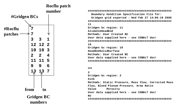
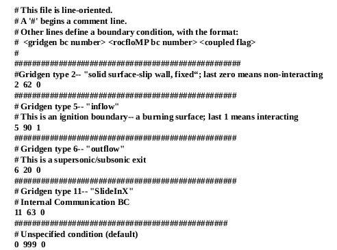
ACM.cgi file also resides at NDAs/Rocflu/Modin and it maps Gridgen BC numbers to Rocflu .bc boundary condition definitions. It is functionally same as Rocflo <casename>.bcmp file. Following image is the example screen shot of ACM.cgi file :
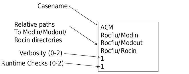
Make sure that you have casename correct in RocfluControl.txt. It is used for Rocprep and Rocflu to know what other files are called. Make sure it is used consistently throughout the files. Normally the other lines will alwayes be the same. Following figure is to help you get the sense of what it should look like :
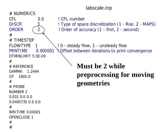
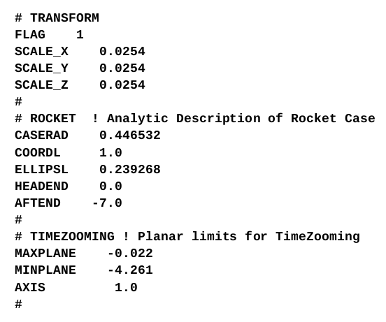
ACM.inp, denoted as labscale.inp in this case, also resides at NDAs/Rocflu/Modin. It controls various parameters of the physcis module. Following images are the example state of ACM.inp.
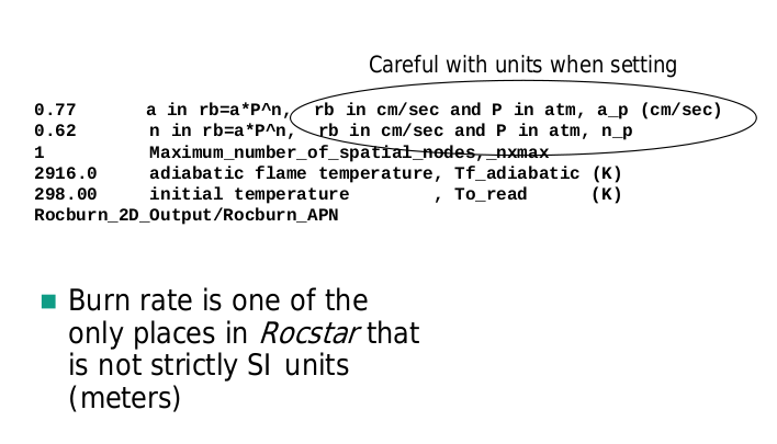
RocstarControl.txt resides at the top directory of the NDA. There should be a directory called Rocman, and in there you can also find RocmanControl.txt. Following images show the important parameters to be set in order to run the example.
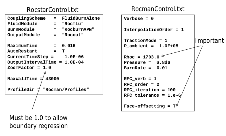
Burn rate is one of the only places in Rocstar that is not strictly SI units (meters)
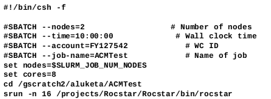
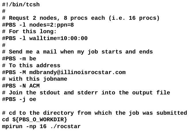
In order to run the problem, you will need to set up a batch-system specific job script for your system. Depends on your choice of the batch-system, the script can look different. Here we provide two examplary script for PBS and SBATCH.
Depending upon your setup, you can "watch" the probe files to monitor progress
The location of this probe is defined in ACM.inp
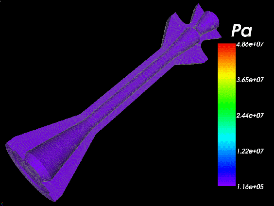
The output can be visualized by using Rocketeer. It can also translate to tecplot format. I need to learn to read the output file naming. Once a checkpoint has occurred, there will be one HDF file per processor per checkpoint.
For Rocflu ACM, pre-run visualization file are available for 0ms, 5ms, 10ms, 14ms. You can load these into Rocketeer from VizData directory
Similar to Rocflu, you export IGES format using CAD software such as Pro/Engineer/ Then you should be able to make some simple geometries in Gridgen. Particularity for Rocflo, it is set block-structured Hex meshes.
Now you should set up NDA with grids and input files. Choose a "casename"; in this case, it should be set ACM. Grid and boundary condition map files. Basic input, boundary conditions, control files.
After all this gets done, we can process and partition using Rocprep on NDA.
Database is made with Pro-Engineer, exported as iges. It gets imported into Gridgen. It is almost always the case that significant clean-up is necessary; Spurious surfaces, lines that don't connect. DB below has many extraneous elements.
Once DB is clean, you can assemble, connectors, domains, and blocks. Some blocking restrictions:
Similar to Rocflu, following requirement should be met for Rocflo boundary conditions:
Running the ACM example problem with Rocflo is almost identical to the method for running with Rocflu. Following the diretions for running the Rocflu problem in the Rocstar Quickstart Guide, the only adjustments that need to be made for running with Rocflo are listed below.
Finally, as in the Rocflu case, the example can be shortened to obtain results in a more timely fashion. Make the following changes to reduce the run time.
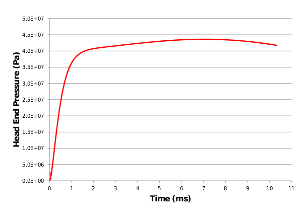
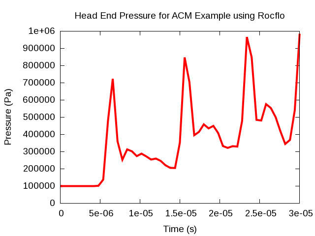
The simulation time can be further shortened if desired. The results for running the simulation with the above changes are shown below for comparison. This graph is generated by plotting column one versus column six from the probe file Rocflo/Modout/ACM.prb_0001.
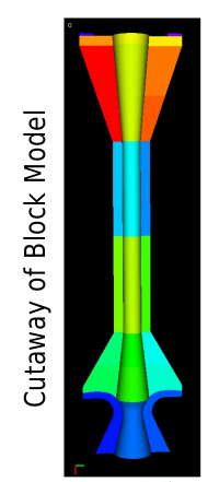
The goal of this example is to assemble and run a fully coupled fluid-solid interaction prblem with significant solid deformation. This problem deals with shock wave propagation causing solid deformation. Rocflo and Rocfrac are used to solve this problem, both using a block-structured, hexahedral grid.
Make sure following file structure is maintained throughout the process:
Shock in a compressible fluid travels at a speed that exceeds the dilational wave speed in a solid


Solid material properties similar to copper
 Fluid material properties modified to get a sound speed similar to

 Causes deformation of the solid due to high pressures behind the shock
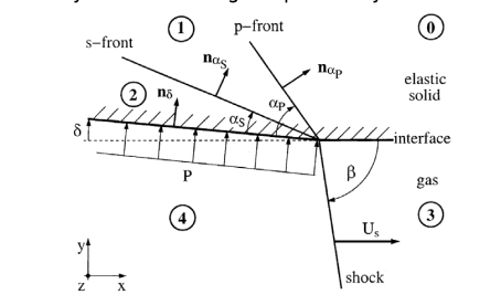
This example can be run in the same manner as the ACM example discussed above. Follow the procedure from the Rocstar Quickstart Guide but using the following commands specific to this example.
This command should generate a directory called SSS_4, which should be ready for running the example. In order to shorten the run time of the example change the following variables.
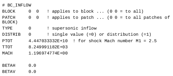
sss.bc is a file that controls the inflow boundary condition. It should be set like following sample image:
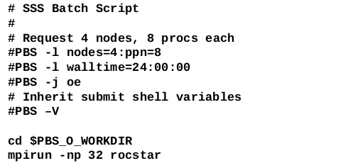
Similar to previous examples, you need to set up a batch-system specific job script for your system. Below is the example batch script for SSS :
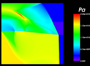
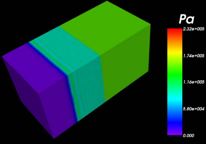
You can visualize the output data with Rocketeer.
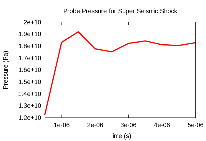
The results for running the simulation with the above changes are shown below for comparison. This graph is generated by plotting column one versus column six from the probe file Rocflo/Modout/sss.prb_0001.
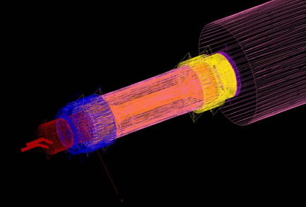
The goal of this example is to assemble and run a fully coupled fluid - solid interaction problem. It consists of an impulsive acceleration of a fluid - solid interface. This example uses the Rocstar packages Rocflo and Rocfrac are used to solve this problem, both using a block-structured, hexahedral grid.
There exists an impulsive acceleration of fluid-solid interface. Rocflo is a block-structured hexahedral grid, 1m cube, pressurized to 1.5*10^5 Pa. Rocfrac is a unstructured 10 node tetrahedral grid, that is 1m cube, initially stress free.
Make sure following file structure is maintained throughout the process:
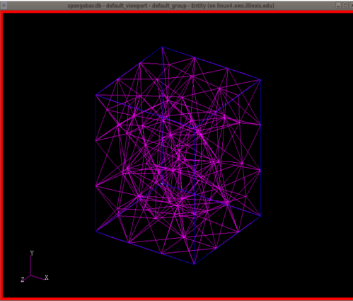
Just like previous examples, DB should be imported into Patron and to create volume mesh. It has both linear and qudratic tetrahedrons and hexahedrons. There is no mixing. Rocfrac mesh should look following :
For Rocflu boundary conditions, following requirement should be met:
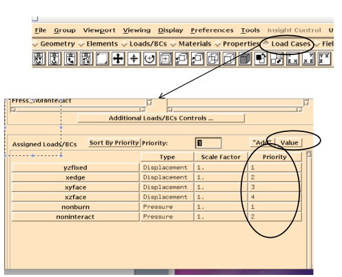
Rocfrac boundary condition priorities must be set in order to determine which BC's take precedence in presence of two or more BC's on a geometrical entitiy.
This example can be run in the same manner as the ACM example discussed above. Follow the procedure from the Rocstar Quickstart Guide but using the following commands specific to this example.
This command should generate a directory called EP_4, which should be ready for running the example. In order to shorten the run time of the example change the following variables.
The results for running the simulation with the above changes are shown below for comparison. This graph is generated by plotting column one versus column six from the probe file Rocflo/Modout/ep.prb_0001.
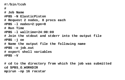
Similar to previous examples, you need to set up a batch-system specific job script for your system. Below is the example batch script for elastic piston example for PBS batch system:
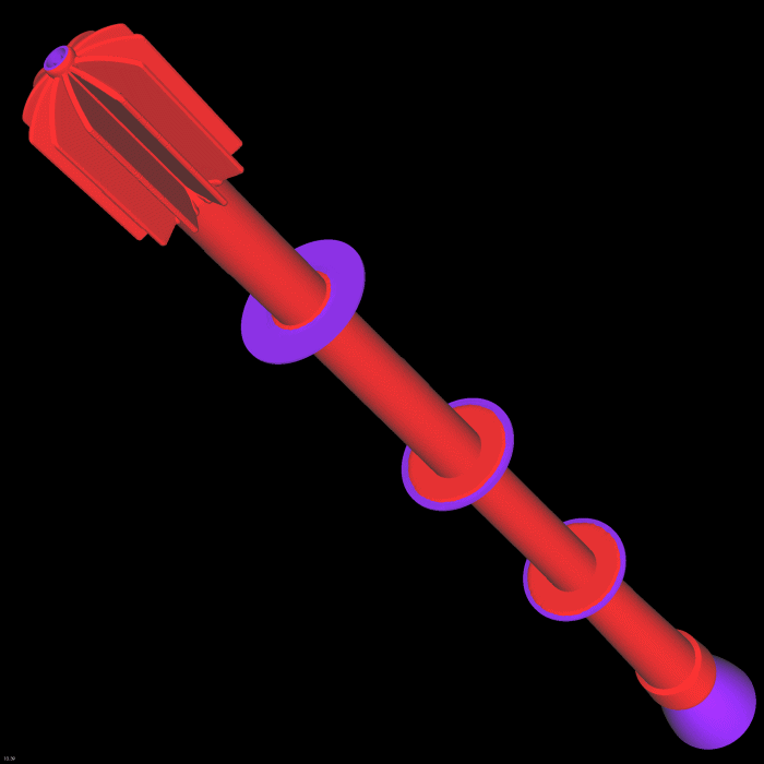
You can visualize the output data with Rocketeer.
For elastic piston, pre-run visualization files are available for one time dump for both Rocflo and Rocfrac. In order to do that, just load one time dump for both into Rocketeer from the VizData directory.
This section is adapted from the SimulationExamples powerpoint.
NASA's reusuable solid rocket motor (RSRM) represents the largest solid rocket motor ever flown. Each motor provides approximately 3-million lb of thrust to lift from the launch pad where the motors burn out approximately two minutes later. The Rocstar suite provides a burnout simulation of this rocket.
The simulation provices unique viewing options such as a propellant/flud interface as well as inhibited surfaces. In terms capabilities, there is a high rate of "time zooming", case constraints, propellant walkback, inhibitor regression and a dynamically changing topology.
 1.8.5
1.8.5